38 how to show alternate data labels in excel
Change Horizontal Axis Values in Excel 2016 - AbsentData 1. Select the Chart that you have created and navigate to the Axis you want to change. 2. Right-click the axis you want to change and navigate to Select Data and the Select Data Source window will pop up, click Edit 3. The Edit Series window will open up, then you can select a series of data that you would like to change. 4. Click Ok 3 Ways to Highlight Every Other Row in Excel - wikiHow Enter the formula to highlight alternating rows. Type the following formula into the typing area: =MOD (ROW (),2)=0 7 Click Format. It's a button on the dialog box. 8 Click the Fill tab. It's at the top of the dialog box. 9 Select a pattern or color for the shaded rows and click OK. You'll see a preview of the color below the formula. 10 Click OK.
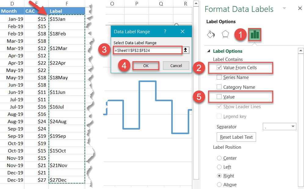
Add Custom Labels to x-y Scatter plot in Excel ... Step 1: Select the Data, INSERT -> Recommended Charts -> Scatter chart (3 rd chart will be scatter chart) Let the plotted scatter chart be Step 2: Click the + symbol and add data labels by clicking it as shown below Step 3: Now we need to add the flavor names to the label.Now right click on the label and click format data labels. Under LABEL OPTIONS select Value From Cells as shown below.

How to show alternate data labels in excel
Add or remove data labels in a chart On the Design tab, in the Chart Layouts group, click Add Chart Element, choose Data Labels, and then click None. Click a data label one time to select all data labels in a data series or two times to select just one data label that you want to delete, and then press DELETE. Right-click a data label, and then click Delete. Dynamically Label Excel Chart Series Lines • My Online ... Hi Mynda - thanks for all your columns. You can use the Quick Layout function in Excel (Design tab of the chart) to do the labels to the right of the lines in the chart. Use Quick Layout 6. You may need to swap the columns and rows in your data for it to show. Then you simply modify the labels to show only the series name. Display every "n" th data label in graphs - Microsoft ... you can use a free tool created by Rob Bovey, called the XY Chart Labeler. With this tool you can assign a range of cells to be the labels for chart series, instead of the Excel defaults. Using a formula, you can have a text show up in every nth cell and then use that range with the XY Chart Labeler to display as the series label.
How to show alternate data labels in excel. How to add data labels from different column in an Excel ... Click any data label to select all data labels, and then click the specified data label to select it only in the chart. 3. Go to the formula bar, type =, select the corresponding cell in the different column, and press the Enter key. See screenshot: 4. Repeat the above 2 - 3 steps to add data labels from the different column for other data points. Two-Level Axis Labels (Microsoft Excel) Excel automatically recognizes that you have two rows being used for the X-axis labels, and formats the chart correctly. (See Figure 1.) Since the X-axis labels appear beneath the chart data, the order of the label rows is reversed—exactly as mentioned at the first of this tip. Figure 1. Two-level axis labels are created automatically by Excel. Edit titles or data labels in a chart - support.microsoft.com The first click selects the data labels for the whole data series, and the second click selects the individual data label. Right-click the data label, and then click Format Data Label or Format Data Labels. Click Label Options if it's not selected, and then select the Reset Label Text check box. Top of Page How To Add Axis Labels In Excel [Step-By-Step Tutorial] Axis labels make Excel charts easier to understand.. Microsoft Excel, a powerful spreadsheet software, allows you to store data, make calculations on it, and create stunning graphs and charts out of your data.. And on those charts where axes are used, the only chart elements that are present, by default, include:
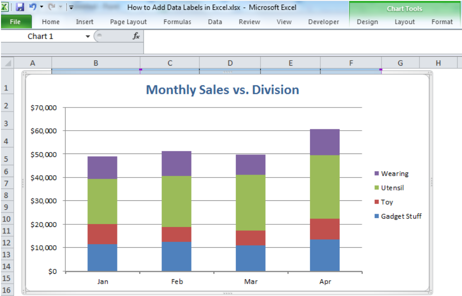
Make your Excel charts easier to read with custom data labels the Legend tab, and clear the Show Legend check box. Click the Data Labels tab and, in the Label Contains section, click the Value check box. Click Next. Click Finish. Right-click one of the data... 10 spiffy new ways to show data with Excel | Computerworld 10 spiffy new ways to show data with Excel ... Right-click the X-axis labels and click Format Axis. In the Axis Options pane, click the Number item and, in Category, select Date from the drop-down Excel Charts: Creating Custom Data Labels - YouTube In this video I'll show you how to add data labels to a chart in Excel and then change the range that the data labels are linked to. This video covers both W... Create Dynamic Chart Data Labels with Slicers - Excel Campus The first step is to create a regular stacked column chart with grand totals above the columns. Jon Peltier has an article that explains how to add the grand totals to the stacked column chart. Step 2: Calculate the Label Metrics The source data for the stacked chart looks like the following.
How to add or move data labels in Excel chart? In Excel 2013 or 2016. 1. Click the chart to show the Chart Elements button . 2. Then click the Chart Elements, and check Data Labels, then you can click the arrow to choose an option about the data labels in the sub menu. See screenshot: In Excel 2010 or 2007. 1. click on the chart to show the Layout tab in the Chart Tools group. See ... How to Use Cell Values for Excel Chart Labels Select range A1:B6 and click Insert > Insert Column or Bar Chart > Clustered Column. The column chart will appear. We want to add data labels to show the change in value for each product compared to last month. Advertisement Select the chart, choose the "Chart Elements" option, click the "Data Labels" arrow, and then "More Options." How to Customize Your Excel Pivot Chart Data Labels - dummies The Data Labels command on the Design tab's Add Chart Element menu in Excel allows you to label data markers with values from your pivot table. When you click the command button, Excel displays a menu with commands corresponding to locations for the data labels: None, Center, Left, Right, Above, and Below. None signifies that no data labels should be added to the chart and Show signifies ... Apply Custom Data Labels to Charted Points - Peltier Tech Click once on a label to select the series of labels. Click again on a label to select just that specific label. Double click on the label to highlight the text of the label, or just click once to insert the cursor into the existing text. Type the text you want to display in the label, and press the Enter key.
Charting in Excel - Adding Data Labels - YouTube
Excel tutorial: How to customize axis labels Now let's customize the actual labels. Let's say we want to label these batches using the letters A though F. You won't find controls for overwriting text labels in the Format Task pane. Instead you'll need to open up the Select Data window. Here you'll see the horizontal axis labels listed on the right. Click the edit button to access the ...
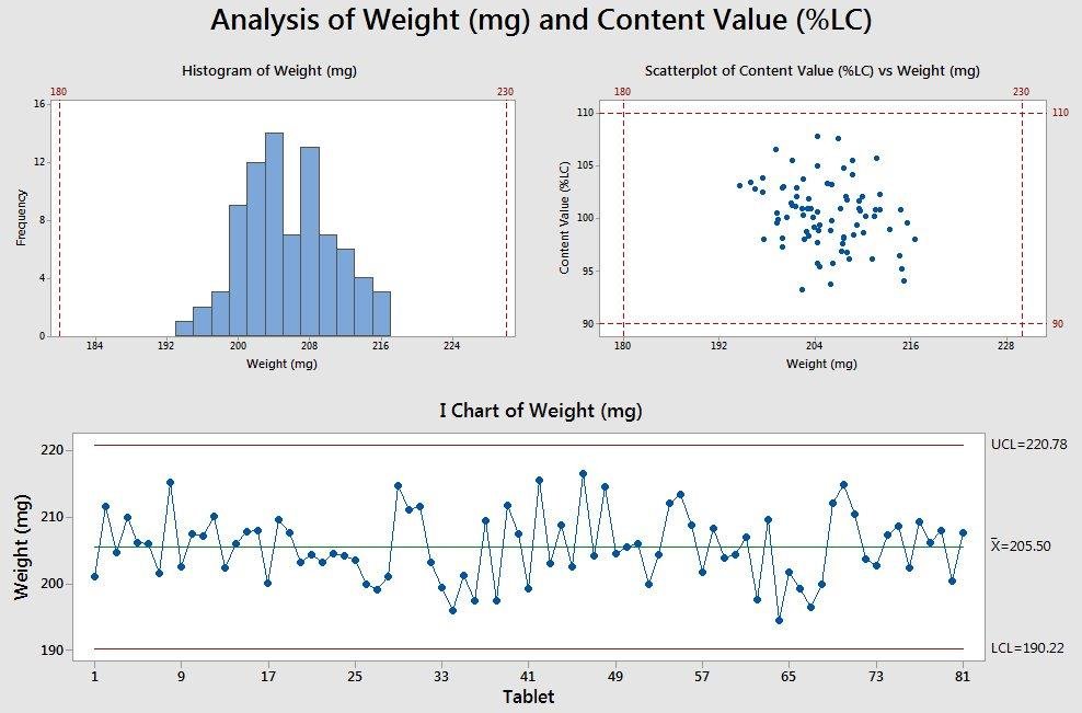
5 Minitab graphs tricks you probably didn’t know about - Master Data Analysis
How to Change Excel Chart Data Labels to Custom Values? Now, click on any data label. This will select "all" data labels. Now click once again. At this point excel will select only one data label. Go to Formula bar, press = and point to the cell where the data label for that chart data point is defined. Repeat the process for all other data labels, one after another. See the screencast. Points to note:
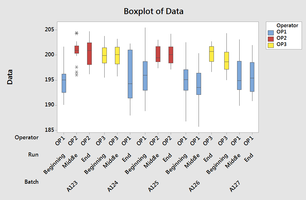
5 Minitab graphs tricks you probably didn’t know about - Master Data Analysis
Chart: Display alternative values as Data Labels or Data ... Joined. Aug 11, 2017. Messages. 1. Aug 11, 2017. #1. Below is my excel chart. I would like to add a "data labels" or "data callouts". As you can see the line is displaying the data from Actual X and Y, but I want to display the DEV values on this line.
How to Add Data Labels in Excel - Excelchat | Excelchat
Alternate row color and column shading in Excel (banded ... Select the range of cells where you want to alternate color rows. Navigate to the Insert tab on the Excel ribbon and click Table, or press Ctrl+T. Done! The odd and even rows in your table are shaded with different colors. The best thing is that automatic banding will continue as you sort, delete or add new rows to your table.
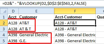
Excel: Show Customer Account & Name - Excel Articles
How to show different fonts for different data labels in ... So far, I've tried using the chart series option "data_labels" a first time at the "add_series" level in order to set the main format for my data labels, and then within each of the "points" in my doughnut chart, I tried including a different version of the "data_labels" option (see code below).
Add or remove data labels in a chart - Office Support
Custom Y-Axis Labels in Excel - PolicyViz 1. Select that column and change it to a scatterplot. 2. Select the point, right-click to Format Data Series and plot the series on the Secondary Axis. 3. Show the Secondary Horizontal axis by going to the Axes menu under the Chart Layout button in the ribbon. (Notice how the point moves over when you do so.) 4.

Format: Chart: Column Chart | Format | Jan's Working with Numbers
Custom data labels in a chart - Get Digital Help Press with right mouse button on on any data series displayed in the chart. Press with mouse on "Add Data Labels". Press with mouse on Add Data Labels". Double press with left mouse button on any data label to expand the "Format Data Series" pane. Enable checkbox "Value from cells".

34 Label In Excel Definition - Labels Database 2020
How to use AutoFill in Excel - all fill handle options ... Go to File / Office button -> Options -> Advanced and find the Cut, copy and paste section. Clear the Show Paste Options buttons when content is pasted check box. In Microsoft Excel, AutoFill is a feature that allows the user to extend a series of numbers, dates, or even text to the necessary range of cells.

How to change data labels position in Excel 2021, right-click the selection >
Excel Charts: Dynamic Label positioning of line series Go to Layout tab, select Data Labels > Right. Right mouse click on the data label displayed on the chart. Select Format Data Labels. Under the Label Options, show the Series Name and untick the Value. You can see that now it's showing the data labels also for zero values. So why does Excel do that?
Enable or Disable Excel Data Labels at the click of a button - How To - PakAccountants.com
Display every "n" th data label in graphs - Microsoft ... you can use a free tool created by Rob Bovey, called the XY Chart Labeler. With this tool you can assign a range of cells to be the labels for chart series, instead of the Excel defaults. Using a formula, you can have a text show up in every nth cell and then use that range with the XY Chart Labeler to display as the series label.
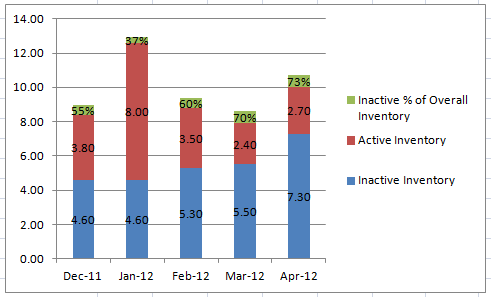
How-to Put Percentage Labels on Top of a Stacked Column Chart - Excel Dashboard Templates
Dynamically Label Excel Chart Series Lines • My Online ... Hi Mynda - thanks for all your columns. You can use the Quick Layout function in Excel (Design tab of the chart) to do the labels to the right of the lines in the chart. Use Quick Layout 6. You may need to swap the columns and rows in your data for it to show. Then you simply modify the labels to show only the series name.
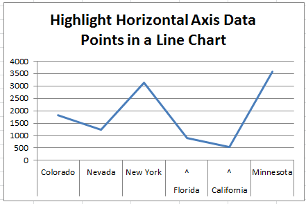
How-to Highlight Specific Horizontal Axis Labels in Excel Line Charts
Add or remove data labels in a chart On the Design tab, in the Chart Layouts group, click Add Chart Element, choose Data Labels, and then click None. Click a data label one time to select all data labels in a data series or two times to select just one data label that you want to delete, and then press DELETE. Right-click a data label, and then click Delete.

Enable or Disable Excel Data Labels at the click of a button - How To - PakAccountants.com
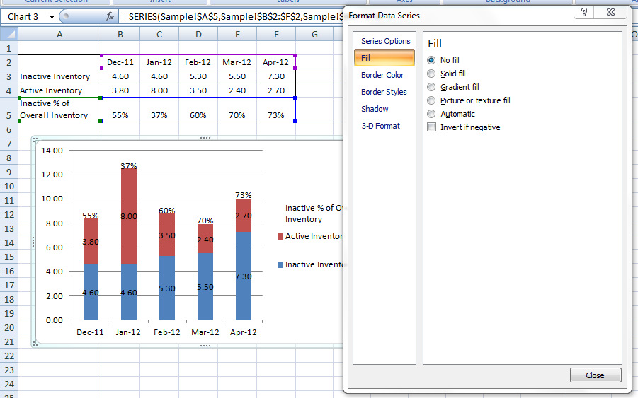
Excel Dashboard Templates How-to Put Percentage Labels on Top of a Stacked Column Chart - Excel ...
How to Create a Step Chart in Excel - Automate Excel
Post a Comment for "38 how to show alternate data labels in excel"