44 excel chart remove data labels
How to Create and Customize a Waterfall Chart in Microsoft ... Select the chart and use the buttons on the right (Excel on Windows) to adjust Chart Elements like labels and the legend, or Chart Styles to pick a theme or color scheme. Select the chart and go to the Chart Design tab. Then, use the tools in the ribbon to select a different layout, change the colors, pick a new style, or adjust your data ... › gantt-chart › how-to-makeExcel Gantt Chart Tutorial + Free Template + Export to PPT Right-click the white chart space and click Select Data to bring up Excel's Select Data Source window. On the left side of Excel's Data Source window, you will see a table named Legend Entries (Series). Click on the Add button to bring up Excel's Edit Series window where you will begin adding the task data to your Gantt chart.
DataLabels.Separator property (Excel) | Microsoft Docs Remarks. If you use a string, you'll get a string as the separator. If you use xlDataLabelSeparatorDefault (= 1) ( XlDataLabelSeparator enumeration), you'll get the default data label separator, which is either a comma or a newline, depending on the data label. When a value of "1" is returned, it indicates that the user has not changed the ...

Excel chart remove data labels
chandoo.org › wp › budget-vs-actual-chart-free-templateFree Budget vs. Actual chart Excel Template - Download May 16, 2018 · Create Budget vs Actual chart with smart labels in Excel – Tutorial. If you are in a hurry to make such a chart, download the template, plug in your values and you are good to go. For instructions on how to create them in Excel, read along. Step 1: Getting the data. Set up your data. I do not want to show data in chart that is "0" (zero ... Chart Tools > Design > Select Data > Hidden and Empty Cells. You can use these settings to control whether empty cells are shown as gaps or zeros on charts. With Line charts you can choose whether the line should connect to the next data point if a hidden or empty cell is found. If you are using Excel 365 you may also see the Show #N/A as an ... Series.DataLabels method (Excel) | Microsoft Docs Return value. Object. Remarks. If the series has the Show Value option turned on for the data labels, the returned collection can contain up to one label for each point. Data labels can be turned on or off for individual points in the series. If the series is on an area chart and has the Show Label option turned on for the data labels, the returned collection contains only a single label ...
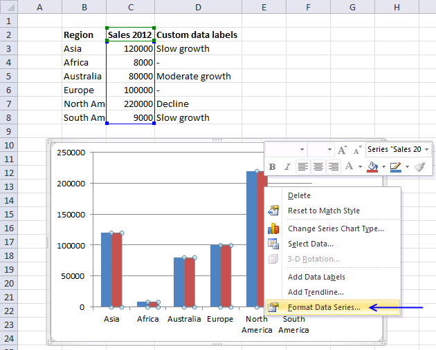
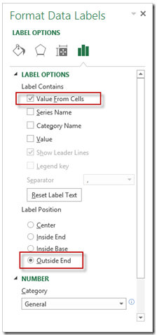
Excel chart remove data labels. How to Add Labels to Scatterplot Points in Excel - Statology Step 3: Add Labels to Points. Next, click anywhere on the chart until a green plus (+) sign appears in the top right corner. Then click Data Labels, then click More Options…. In the Format Data Labels window that appears on the right of the screen, uncheck the box next to Y Value and check the box next to Value From Cells. Bar Chart in Excel - Types, Insertion, Formatting - Excel ... To insert a bar chart from this data:-. Select the source data A1:B13. Go to the Insert tab on the ribbon. Click on the Recommended Charts button, this opens the Insert Chart dialog box. Navigate to the All Charts tab and choose the Clustered Bar Chart. Click Ok. This inserts the bar chart as shown in the preview. support.microsoft.com › en-us › officeAdd or remove a secondary axis in a chart in Excel In the chart, select the data series that you want to plot on a secondary axis, and then click Chart Design tab on the ribbon. For example, in a line chart, click one of the lines in the chart, and all the data marker of that data series become selected. How to Create and Customize a Treemap Chart in Microsoft Excel Select the data for the chart and head to the Insert tab. Click the "Hierarchy" drop-down arrow and select "Treemap.". The chart will immediately display in your spreadsheet. And you can see how the rectangles are grouped within their categories along with how the sizes are determined. In the screenshot below, you can see the largest ...
How to make shading on Excel chart and move x axis labels ... In the Change Chart Type dialog, change the chart type for the new series to Stacked Area. Change the color from whatever Excel decides to yellow. Finally, remove the new series form the legend. See the attached version. Removing gaps between bars in an Excel chart ... Not everyone likes this default appearance, but fortunately it is possible to change the size of the gaps between bars and even remove them altogether. 1. Open the Format Data Series task pane. Right-click on one of the bars in your chart and click Format Data Series from the shortcut menu. The Format Data Series task pane appears on the right ... Format Chart Axis in Excel - Axis Options (Format Axis ... Formatting a Chart Axis in Excel includes many options like Maximum / Minimum Bounds, Major / Minor units, Display units, Tick Marks, Labels, Numerical Format of the axis values, Axis value/text direction, and more. However, there are a lot more formatting options for the chart axis, in this blog, we will be working with the axis options and ... Excel Waterfall Chart: How to Create One That Doesn't Suck Click inside the data table, go to " Insert " tab and click " Insert Waterfall Chart " and then click on the chart. Voila: OK, technically this is a waterfall chart, but it's not exactly what we hoped for. In the legend we see Excel 2016 has 3 types of columns in a waterfall chart: Increase. Decrease.
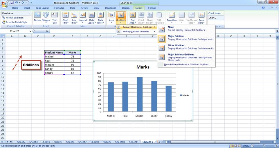
How to Print Labels from Excel - Lifewire Select Mailings > Write & Insert Fields > Update Labels . Once you have the Excel spreadsheet and the Word document set up, you can merge the information and print your labels. Click Finish & Merge in the Finish group on the Mailings tab. Click Edit Individual Documents to preview how your printed labels will appear. Select All > OK . How to Move Excel Pivot Table Labels Quick Tricks Use Menu Commands to Move Label. To move a pivot table label to a different position in the list, you can use commands in the right-click menu: Right-click on the label that you want to move. Click the Move command. Click one of the Move subcommands, such as Move [item name] Up. The existing labels shift down, and the moved label takes its new ... Controlling Chart Gridlines (Microsoft Excel) In the Current Selection group, use the drop-down list to choose the gridlines you want to control. Click the Format Selection tool, also within the Current Selection group. Excel displays a Format task pane at the right side of the program window. Use the controls in the task pane to make changes to the gridlines, as desired. Close the task pane. Clutter-Free: One of the 3 Cs for Better Charts Depending on the situation, you might be able to remove those visual elements and simply use data labels. For example, let's imagine we redesigned an enterprise product website. We increased average monthly lead form submissions from 1232 to 1848. By default, Excel gives us a chart with grid lines, a y-axis, and grid line labels from 0 to 2000.
How to Add Data Labels to an Excel 2010 Chart - dummies
Copy Pivot Chart messes up Data Labels - Microsoft Community I am trying to copy a Pivot Chart and paste it into Power Point. What happens is that Data-Labels that have been deleted in the excel (like 0%) reappear when pasting. This happens regardless of copied as object or picture/ pasted as object or picture. The funny thing is: When I paste in PowerPoint as object, THEN delete the labels, then copy ...

How to Add Data Labels in Excel - Excelchat | Excelchat
Modifying Axis Scale Labels (Microsoft Excel) Follow these steps: Create your chart as you normally would. Double-click the axis you want to scale. You should see the Format Axis dialog box. (If double-clicking doesn't work, right-click the axis and choose Format Axis from the resulting Context menu.) Make sure the Number tab is displayed. (See Figure 1.)
Add or remove data labels in a chart - Office Support
› documents › excelHow to wrap X axis labels in a chart in Excel? Some users may want to wrap the labels in the chart axis only, but not wrap the label cells in the source data. Actually, we can replace original labels cells with formulas in Excel. For example, you want to wrap the label of "OrangeBBBB" in the axis, just find out the label cell in the source data, and then replace the original label with the ...
Custom data labels in a chart | Get Digital Help - Microsoft Excel resource
Remove one label from Multi-label axis in a Pivot Chart Hi, I'm charting a Pivot table and have multiple labels in my horizontal x-axis. From the Pivot table, first column is a label and the second column is a date, and then it's the data for those two. When I chart this and add the data labels to the chart, it is showing the date the long way, vertical 90 degrees, so it fits, but the label is showing horizontally, so it doesn't fit and overlaps ...

How to Add Data Labels to your Excel Chart in Excel 2013 - YouTube
Prevent Overlapping Data Labels in Excel Charts - Peltier Tech Overlapping Data Labels. Data labels are terribly tedious to apply to slope charts, since these labels have to be positioned to the left of the first point and to the right of the last point of each series. This means the labels have to be tediously selected one by one, even to apply "standard" alignments.

Microsoft Excel Tutorials: The Chart Layout Panels
How to remove text or character from cell in Excel ... Select a range of cells where you want to remove a specific character. Press Ctrl + H to open the Find and Replace dialog. In the Find what box, type the character. Leave the Replace with box empty. Click Replace all. As an example, here's how you can delete the # symbol from cells A2 through A6.
Basic Excel Chart Formatting - MS Excel Charting Tutorial Part 4 | Vertical Horizons
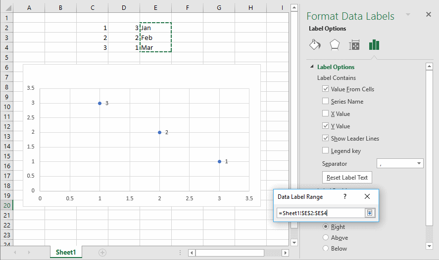
How to Find, Highlight, and Label a Data Point in Excel ... By default, the data labels are the y-coordinates. Step 3: Right-click on any of the data labels. A drop-down appears. Click on the Format Data Labels… option. Step 4: Format Data Labels dialogue box appears. Under the Label Options, check the box Value from Cells . Step 5: Data Label Range dialogue-box appears.

Elements of an Excel Chart | ExcelDemy.com
Excel Pivot Table Filter and Label Formatting - Microsoft ... Excel 2016. Images of 2 separate workbooks, each with a data table, pivot table and pivot chart, the one on the right created by copy & paste of the one on the left. The one on the right changed: X axis labels on the pivot chart don't have the multi-level option. Also, unlike the original on the left, there is now a filter button for the chart.
How-to Use Data Labels from a Range in an Excel Chart - Excel Dashboard Templates
Show/Hide Field Headers in Excel Pivot Tables | MyExcelOnline DOWNLOAD EXCEL WORKBOOK. This is our pivot table. And you can see the 2 field headers on top: STEP 1: Go to PivotTable Analyze > Show > Field Headers. Click on it to hide the field headers: And they are now hidden! You can click on the same button to show them again. The headers will be visible again!
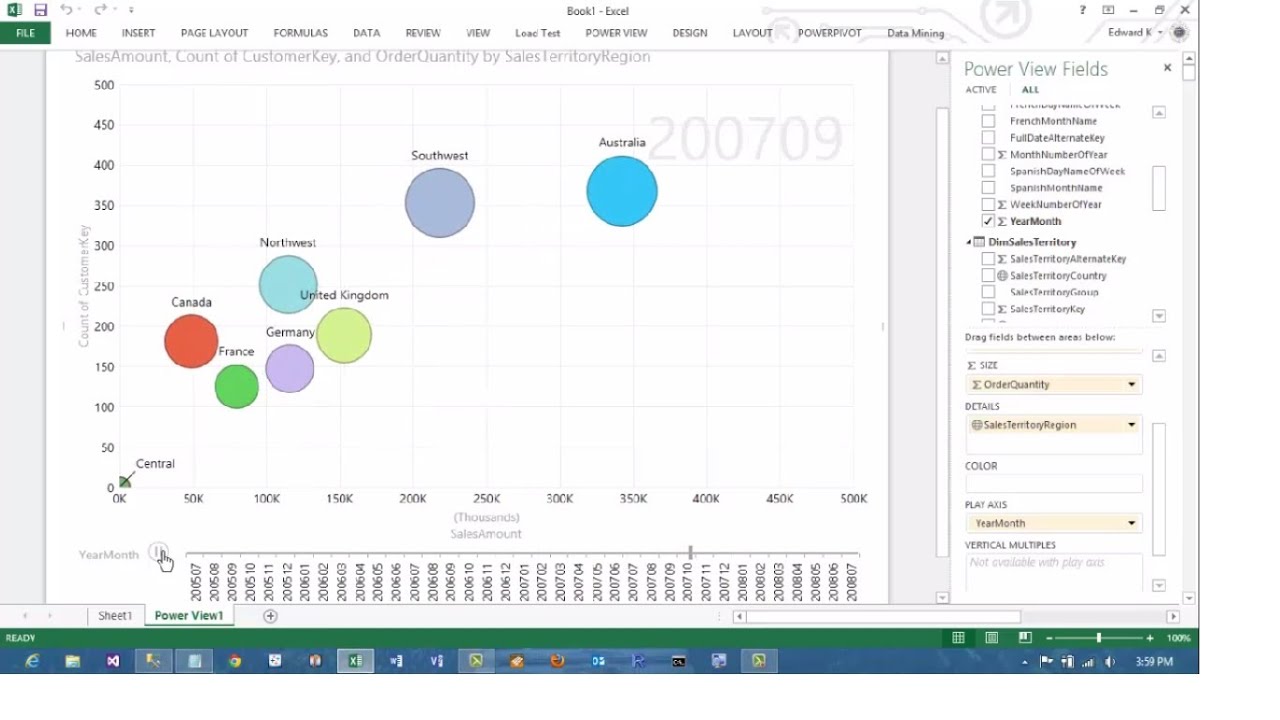
Excel 2013 PowerView Animated Scatterplot/Bubble Chart Business Intelligence Tutorial - YouTube
Custom Excel number format - Ablebits How to create a custom number format in Excel. To create a custom Excel format, open the workbook in which you want to apply and store your format, and follow these steps: Select a cell for which you want to create custom formatting, and press Ctrl+1 to open the Format Cells dialog. Under Category, select Custom.
Custom data labels in a chart
How to create pill charts in Excel Creating pill charts. 1. Add chart. Start by creating a stacked bar or column chart from the data with helper columns. 2. Remove unnecessary elements. Once the chart is ready, remove the legend and the value axis items. You can either click on the object and press Delete button or use the Chart Elements (Plus at the right side) button to remove ...
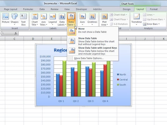
How to Add a Data Table to an Excel 2007 Chart - dummies
How to Use Excel Pivot Table Label Filters Watch the steps in this short video, and the written instructions are below the video. Play. To change the Pivot Table option to allow multiple filters: Right-click a cell in the pivot table, and click PivotTable Options. Click the Totals & Filters tab Under Filters, add a check mark to 'Allow multiple filters per field.'.

How to get Excel Chart Columns with no gaps • AuditExcel.co.za
Excel: How to Create a Bubble Chart with Labels - Statology Step 3: Add Labels. To add labels to the bubble chart, click anywhere on the chart and then click the green plus "+" sign in the top right corner. Then click the arrow next to Data Labels and then click More Options in the dropdown menu: In the panel that appears on the right side of the screen, check the box next to Value From Cells within ...

Quickly Add Accumulated Total Line To A Chart In Excel
excelchamps.com › excel-charts › milestone-chartHow to Create a Milestone Chart in Excel in 3 Steps ... Steps to Create a Milestone Chart in Excel. I have split the entire process into three steps to make it easy for you to understand. 1. Set Up Data. You can easily set up your data for this chart. Make sure to arrange your data like below data table.

Do My Excel Blog: How to hide the zero percent labels in an Excel pie chart
excel - Adding Data Label To Chart Based On X Values ... Here's my setup. Categories, including maybe "Red" in column A, Values in column B, and chart labels in column C. In cell C2 I'm using a formula like this: =IF (A2="Red","Label Text Here","") so there is only text in that column if the X value is "Red". My chart plots columns A and B of the data range. I added data labels, then formatted the ...
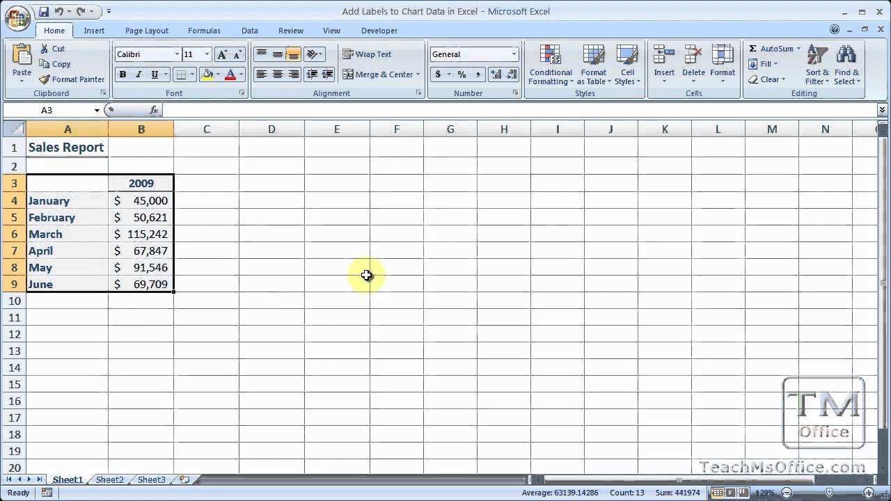
Add Labels to Chart Data in Excel - YouTube
How To Add Axis Labels In Excel [Step-By-Step Tutorial] First off, you have to click the chart and click the plus (+) icon on the upper-right side. Then, check the tickbox for 'Axis Titles'. If you would only like to add a title/label for one axis (horizontal or vertical), click the right arrow beside 'Axis Titles' and select which axis you would like to add a title/label. Editing the Axis Titles

Microsoft Excel Tutorials: The Chart Layout Panels
› documents › excelHow to create progress bar chart in Excel? - ExtendOffice Then close the Format Data Series pane, and then click to select the whole chart, and click Design > Add Chart Element > Data Labels > Inside Base, all data labels have been inserted into the chart as following screenshot shown: 5. And then you should delete other data labels and only keep the current data labels as following screenshot shown: 6.
Post a Comment for "44 excel chart remove data labels"