39 excel chart ignore blank axis labels
Unlink Chart Data - Peltier Tech It's easy to link many of a chart's text elements to a worksheet range. Select the text element, click in the formula bar, type = and click on the cell or range containing the text you want displayed. The result is a link formula like =Sheet1!$A$1, and the text element updates dynamically to display whatever is in the reference. - Automate Excel Chart Axis Text Instead of Numbers: Copy Chart Format: Create Chart with Date or Time: Curve Fitting: Export Chart as PDF: Add Axis Labels: Add Secondary Axis: Change Chart Series Name: Change Horizontal Axis Values: Create Chart in a Cell: Graph an Equation or Function: Overlay Two Graphs: Plot Multiple Lines: Rotate Pie Chart: Switch X and Y ...
Excel Graph should not have trailing empty cells take up space on axis Edit the graph: Right-click on the graph and select 'Select Data'. Select a series and click 'Edit'. In the 'Series Values' box, enter something like: ='Spread Sheet Name.xlsx'!RangeName. Where 'Spread Sheet Name' is your spreadsheet name and 'RangeName' is your range name. excel graph trailing. Share.

Excel chart ignore blank axis labels
Learn To Excel At Excel With Our Videos, Downloads, Tips and Excel ... Excel Resources If you are looking to Excel At Excel then this is a great place to start. For recommended courses, books, reviews and Excel news Most Recent Publications. Delete Excel Rows That Do Not Contain Specified String-01/05/2022. Convert A Range Of Cells To Lower Case With An Excel Macro - 24/04/2022. Edit Multiple Formulas In Excel - FAST -22/04/2022 peltiertech.com › broken-y-axis-inBroken Y Axis in an Excel Chart - Peltier Tech Nov 18, 2011 · For the many people who do want to create a split y-axis chart in Excel see this example. Jon – I know I won’t persuade you, but my reason for wanting a broken y-axis chart was to show 4 data series in a line chart which represented the weight of four people on a diet. One person was significantly heavier than the other three. excel - VBA for Dynamic Chart Data with N/A or Dynamic Range - Stack ... The chart is not so complex. But your data is not laid out optimally. The #N/A in the Y value columns will not plot points, but all the blanks in the date column are messing you up. Delete all those rows below row 33. They are what is killing the chart. Now select the range A7:R33, and on the Insert tab of the ribbon, choose Table.
Excel chart ignore blank axis labels. Use defined names to automatically update a chart range - Office Select cells A1:B4. On the Insert tab, click a chart, and then click a chart type. Click the Design tab, click the Select Data in the Data group. Under Legend Entries (Series), click Edit. In the Series values box, type =Sheet1!Sales, and then click OK. Under Horizontal (Category) Axis Labels, click Edit. Chart suddenly ignoring "do not overlap legend" setting Re: Chart suddenly ignoring "do not overlap legend" setting. Hello Andy, I tried that but it does not yield the same result as it would when I do it manually. If I manually change the pot area width, then obvisouly it works. But when I run the exact same code the macro recorder recorded, it will change the width and stay aligned on the right. A Solution to Tableau Line Charts with Missing Data Points Yes! The obvious answer is to use the IFNULL function, and this would work great if our data looked like this: But our data doesn't look like this, so the IFNULL function won't work as there are no nulls in the data. As mentioned above, we don't have null values, we have no data. This is a critical and often misunderstood point. The Solution How to Use Excel Pivot Table Label Filters Right-click a cell in the pivot table, and click PivotTable Options. In the PivotTable Options dialog box, click the Totals & Filters tab In the Filters section, add a check mark to 'Allow multiple filters per field.' Click the OK button, to apply the setting and close the dialog box. Quick Way to Hide or Show Pivot Items
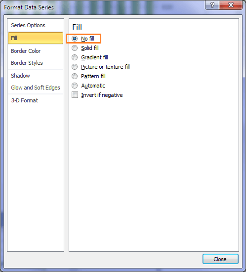
clickup.com › blog › gantt-chart-excelHow To Make A Gantt Chart In Excel? (With Templates!) Well, Excel has some significant drawbacks that you can’t ignore. 3 Drawbacks Of An Excel Gantt Chart. A spreadsheet is no one’s first love. 💔. And making Gantt charts on it? Frankly, you don’t want to even try. Here are some drawbacks that will explain why creating an Excel Gantt chart is not an ideal option. 1. No workflow capabilities How to Remove Duplicates from the Pivot Table - Excel Tutorials When we remove the blank sign and go to our Pivot Table, select it, go to PivotTable Tools >> Analyze >> Refresh, our data will now change: Now we only have one "Red" color in our Spring Color column. Remove Duplicates with Data Formatting There could be one more reason why the Pivot Table is showing duplicates. Removing gaps between bars in an Excel chart - TheSmartMethod.com 1. Open the Format Data Series task pane Right-click on one of the bars in your chart and click Format Data Series from the shortcut menu. The Format Data Series task pane appears on the right-hand side of the screen, offering many different options. Excel Pivot Table Report Filter Tips and Tricks Right-click a cell in the pivot table, and click Pivot Table Options. On the Layout & Format tab, click the drop down arrow beside 'Display Fields in Report Filter Area'. Click 'Over, Then Down'. In the 'Report filter fields per row' box, select the number of filters to go across each row.
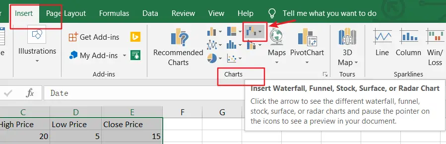
Empty and null data points in paginated report charts - Microsoft ... Charts process empty values differently depending on the specified chart type: If the chart type is a linear chart type (bar, column, scatter, line, area, range), empty values are displayed as empty spaces or "gaps" in the chart. If you want to indicate empty points, you must add empty point placeholders. Excel Waterfall Chart Template - Corporate Finance Institute Select the Horizontal axis, right-click and go to Select Data. Select cell C5 to C11 as the Horizontal axis labels. Right-click on the horizontal axis and select Format Axis. Under Axis Options -> Labels, choose Low for the Label Position. Change Chart Title to "Free Cash Flow.". Remove gridlines and chart borders to clean up the waterfall ... Date Axis in Excel Chart is wrong - AuditExcel.co.za In order to do this you just need to force the horizontal axis to treat the values as text by right clicking on the horizontal axis, choose Format Axis Change Axis Type to be Text Note that you immediately lose the scaling options and the date scale puts in exactly what is in the data, onto the horizontal axis. How to get a chart to ignore blank cells in data? I'd like the chart to ignore the blanks completely - as you can see, it currently pots those blank cells at zero: ... The line has been removed but the chart doesn't resize to only show the data - there's a large blank. The X axis is dates, so the #N/A cells are still registering those dates. ... We have a great community of people providing ...
24 How To Label A Chart In Excel - Modern Label Ideas
How to freeze panes in Excel (lock rows and columns) - Ablebits To lock several rows and columns at a time, select a cell below the last row and to the right of the last column you want to freeze. For example, to freeze the top row and first column , select cell B2, go to the View tab and click Freeze Panes under Freeze Panes:

35 How To Label Axes On Excel 2010 - Labels Database 2020
› shortcuts › trace-precedentsExcel Trace Precedents or Dependents Shortcuts - Automate Excel Break Chart Axis: Calculate Area Under Curve: Plot Residuals: Change Bar Chart Width: Change Chart Colors: Chart Axis Text Instead of Numbers: Copy Chart Format: Create Chart with Date or Time: Curve Fitting: Export Chart as PDF: Add Axis Labels: Add Secondary Axis: Change Chart Series Name: Change Horizontal Axis Values: Create Chart in a Cell ...

Excel Chart - Do not Hide Horizontal Data Label - Stack Overflow
› solutions › yamazumiYamazumi Chart Excel template - Systems2win Chart Labels. At any time, you can change the details that get displayed . in the Chart Labels for each Work Element in your stacked bar chart. At any time, you can change the details show in the Chart Labels for every Work Element in your Yamazumi Chart There are 4 pink cells where you can use the dropdown lists to choose TRUE or FALSE

31 Excel Chart Axis Label - Labels For Your Ideas
How to Create A Timeline Graph in Excel [Tutorial & Templates] Click the vertical Axis Major Gridlines on the chart and hit delete on the keyboard. This clears the lines from the chart plot area. Then change the scales on both vertical axes. To do this, right click on an axis, select Format Axis. Under axis options on the sidebar, change the Bounds to Minimum -20 and Maximum +20.

Excel Custom Chart Labels • My Online Training Hub
Best Types of Charts in Excel for Data Analysis ... - Optimize Smart #1 Use a bar chart whenever the axis labels are too long to fit in a column chart: What are the different types of bar charts? Horizontal bar charts - Represent the data horizontally. The data categories are shown on the vertical axis, and data values are shown on the horizontal axis. Vertical bar charts - Also called a column chart.
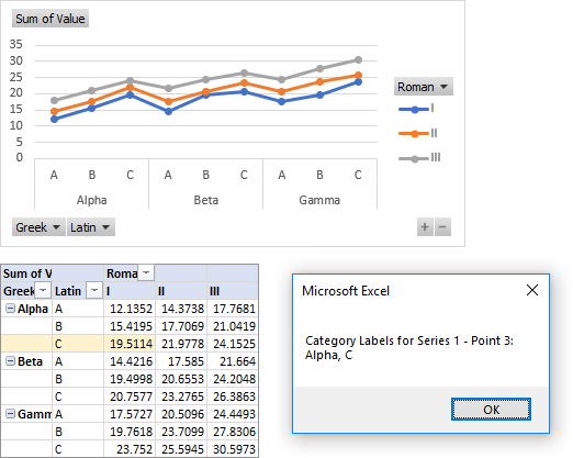
Extract Labels from Category Axis in an Excel Chart (VBA) - Peltier Tech Blog
How to get a chart to ignore blank cells in data? | Page 2 | MrExcel ... But if the value in the date column and the value in the ROI column are both #N/A, then there will be no points for that data pair, no dates, and no space along the axis. In the second data range and chart below, I've inserted another column for the dates in the specific chart. The formula in cell C14 is:.
How to Warp X-Axis labels in Excel - Free Excel Tutorial
Make Excel Chart Gridlines Square - Peltier Tech There is a strange blank edge to the chart, but you could make it look less strange by formatting the plot area border to match the axes. Let's try with another chart. This is like the first, but the X values are twice as large as before, leading to a different scale. This is the resulting chart.

31 Excel Chart Label Axis - Label Design Ideas 2020
How to Add a Vertical Line to Charts in Excel - Statology Step 3: Create Line Chart with Vertical Line. Lastly, we can highlight the cells in the range A2:C14, then click the Insert tab along the top ribbon, then click Scatter with Smooth Lines within the Charts group: The following line chart will be created: Notice that the vertical line is located at x = 6, which we specified at the end of our ...
How to Create a Stock Chart (Open-High-Low-Close) in Excel - Free Excel Tutorial
I do not want to show data in chart that is "0" (zero) To access these options, select the chart and click: Chart Tools > Design > Select Data > Hidden and Empty Cells You can use these settings to control whether empty cells are shown as gaps or zeros on charts. With Line charts you can choose whether the line should connect to the next data point if a hidden or empty cell is found.
Excel Custom Chart Labels • My Online Training Hub
stackoverflow.com › questions › 15013911Creating a chart in Excel that ignores #N/A or blank cells As there is a difference between a Line chart and a Stacked Line chart. The stacked one, will not ignore the 0 or blank values, but will show a cumulative value according with the other legends. Simply right click the graph, click Change Chart Type and pick a non-stacked chart.
Text Labels on a Horizontal Bar Chart in Excel - Peltier Tech Blog
Excel Waterfall Chart: How to Create One That Doesn't Suck Click inside the data table, go to " Insert " tab and click " Insert Waterfall Chart " and then click on the chart. Voila: OK, technically this is a waterfall chart, but it's not exactly what we hoped for. In the legend we see Excel 2016 has 3 types of columns in a waterfall chart: Increase. Decrease.
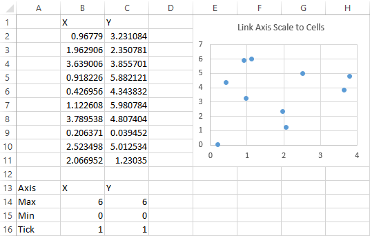
Link Excel Chart Axis Scale to Values in Cells - Peltier Tech Blog
How to Change the X-Axis in Excel - Alphr Follow the instructions to change the text-based X-axis intervals: Open the Excel file and select your graph. Now, right-click on the Horizontal Axis and choose Format Axis… from the menu. Select...
Post a Comment for "39 excel chart ignore blank axis labels"