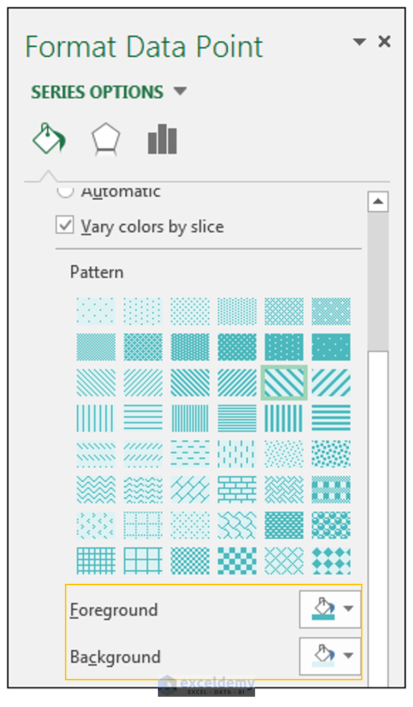
43 pie chart excel labels
Add Labels with Lines in an Excel Pie Chart (with Easy Steps) To enables the data labels on the pie chart, Click on the Pie Chart first. Then click on the plus icon at the top-right corner of the pie chart. Now select Data Labels in the Chart Elements list. After that, you will see a variety of data labels position option such as, Center Inside End Outside End Best Fit Data callout Add a pie chart - support.microsoft.com Click Insert > Insert Pie or Doughnut Chart, and then pick the chart you want. Click the chart and then click the icons next to the chart to add finishing touches: To show, hide, or format things like axis titles or data labels, click Chart Elements . To quickly change the color or style of the chart, use the Chart Styles .
How to Make a Pie Chart in Excel (Only Guide You Need) Now select the cells A3 to B8 and right-click on your mouse and press on to Quick Analysis. In the Quick Analysis, you will find many options to analyze your data. From there select Charts and press on to Pie. You can also insert the pie chart directly from the insert option on top of the excel worksheet.

Pie chart excel labels
How to Make a PIE Chart in Excel (Easy Step-by-Step Guide) Here are the steps to format the data label from the Design tab: Select the chart. This will make the Design tab available in the ribbon. In the Design tab, click on the Add Chart Element (it's in the Chart Layouts group). Hover the cursor on the Data Labels option. Select any formatting option from the list. How to Create a Pie Chart in Excel | Smartsheet To create a pie chart in Excel 2016, add your data set to a worksheet and highlight it. Then click the Insert tab, and click the dropdown menu next to the image of a pie chart. Select the chart type you want to use and the chosen chart will appear on the worksheet with the data you selected. How to display leader lines in pie chart in Excel? - ExtendOffice To display leader lines in pie chart, you just need to check an option then drag the labels out. 1. Click at the chart, and right click to select Format Data Labels from context menu. 2. In the popping Format Data Labels dialog/pane, check Show Leader Lines in the Label Options section. See screenshot: 3.
Pie chart excel labels. How to Create and Format a Pie Chart in Excel - Lifewire Select the plot area of the pie chart. Right-click the chart. Select Add Data Labels . Select Add Data Labels. In this example, the sales for each cookie is added to the slices of the pie chart. Change Colors When a chart is created in Excel, or whenever an existing chart is selected, two additional tabs are added to the ribbon. Create a Pie Chart in Excel (In Easy Steps) Select the pie chart. 9. Click the + button on the right side of the chart and click the check box next to Data Labels. 10. Click the paintbrush icon on the right side of the chart and change the color scheme of the pie chart. Result: 11. Right click the pie chart and click Format Data Labels. 12. Edit titles or data labels in a chart - support.microsoft.com On a chart, click the label that you want to link to a corresponding worksheet cell. On the worksheet, click in the formula bar, and then type an equal sign (=). Select the worksheet cell that contains the data or text that you want to display in your chart. You can also type the reference to the worksheet cell in the formula bar. How to Edit Pie Chart in Excel (All Possible Modifications) How to Edit Pie Chart in Excel 1. Change Chart Color 2. Change Background Color 3. Change Font of Pie Chart 4. Change Chart Border 5. Resize Pie Chart 6. Change Chart Title Position 7. Change Data Labels Position 8. Show Percentage on Data Labels 9. Change Pie Chart's Legend Position 10. Edit Pie Chart Using Switch Row/Column Button 11.
How to Show Pie Chart Data Labels in Percentage in Excel Click anywhere on the Pie Chart, and the Chart Elements icon will appear on the right side. Next, click on it and then click on the right arrow icon beside the Data Labels option. Later, select More Options from the appeared menu. Soon after, you will get the Format Data Labels field on the right side of your sheet. Pie Chart in Excel - Inserting, Formatting, Filters, Data Labels Right click on the Data Labels on the chart. Click on Format Data Labels option. Consequently, this will open up the Format Data Labels pane on the right of the excel worksheet. Mark the Category Name, Percentage and Legend Key. Also mark the labels position at Outside End. This is how the chark looks. Formatting the Chart Background, Chart Styles How to Make a Pie Chart in Excel & Add Rich Data Labels to The Chart! Creating and formatting the Pie Chart 1) Select the data. 2) Go to Insert> Charts> click on the drop-down arrow next to Pie Chart and under 2-D Pie, select the Pie Chart, shown below. 3) Chang the chart title to Breakdown of Errors Made During the Match, by clicking on it and typing the new title. Change the format of data labels in a chart To get there, after adding your data labels, select the data label to format, and then click Chart Elements > Data Labels > More Options. To go to the appropriate area, click one of the four icons ( Fill & Line, Effects, Size & Properties ( Layout & Properties in Outlook or Word), or Label Options) shown here.
How to Change Font Size of Data Labels in Excel - ExcelDemy After getting the proper pie chart, select the whole chart and choose Data Labels from the Chart Elements. Then, select the data and go to the Home tab. Afterward, choose the proper font size according to your need. In the end, the following result will come up on the screen. Read More: What Are Data Labels in Excel (Uses & Modifications) Pie of Pie Chart in Excel - Inserting, Customizing, Formatting Inserting a Pie of Pie Chart. Let us say we have the sales of different items of a bakery. Below is the data:-. To insert a Pie of Pie chart:-. Select the data range A1:B7. Enter in the Insert Tab. Select the Pie button, in the charts group. Select Pie of Pie chart in the 2D chart section. How to Show Percentage in Excel Pie Chart (3 Ways) To active the Format Data Labels window, follow the simple steps below. Steps: Click on the pie chart to make it active. Now, click the Chart Elements button ( the Plus + sign at the top right corner of the pie chart). Click the Data Labels checkbox which is unchecked by After that, click the Right Arrow sign at the right of the Data Labels Pie Chart in Excel | How to Create Pie Chart - EDUCBA Pie Chart in Excel is used for showing the completion or main contribution of different segments out of 100%. It is like each value represents the portion of the Slice from the total complete Pie. For Example, we have 4 values A, B, C and D.

31 Label Pie Chart Excel - Labels For You
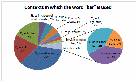
Pie Chart Best Fit Labels Overlapping - VBA Fix Hi @CWTocci. I hope you are doing well. I created attached Pie chart in Excel with 31 points and all labels are readable and perfectly placed. It is created from few clicks without VBA using data visualization tool in Excel. Data Visualization Tool For Excel. Data Visualization Tool For Google Sheets. It has auto cluttering effect to adjust ...
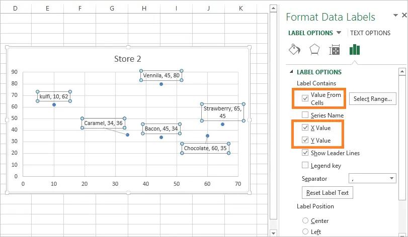
Add Custom Labels to x-y Scatter plot in Excel - DataScience Made Simple
How to hide zero data labels in chart in Excel? - ExtendOffice If you want to hide zero data labels in chart, please do as follow: 1. Right click at one of the data labels, and select Format Data Labels from the context menu. See screenshot: 2. In the Format Data Labels dialog, Click Number in left pane, then select Custom from the Category list box, and type #"" into the Format Code text box, and click Add button to add it to Type list box.
Pie chart and label
How to display leader lines in pie chart in Excel? - ExtendOffice To display leader lines in pie chart, you just need to check an option then drag the labels out. 1. Click at the chart, and right click to select Format Data Labels from context menu. 2. In the popping Format Data Labels dialog/pane, check Show Leader Lines in the Label Options section. See screenshot: 3.
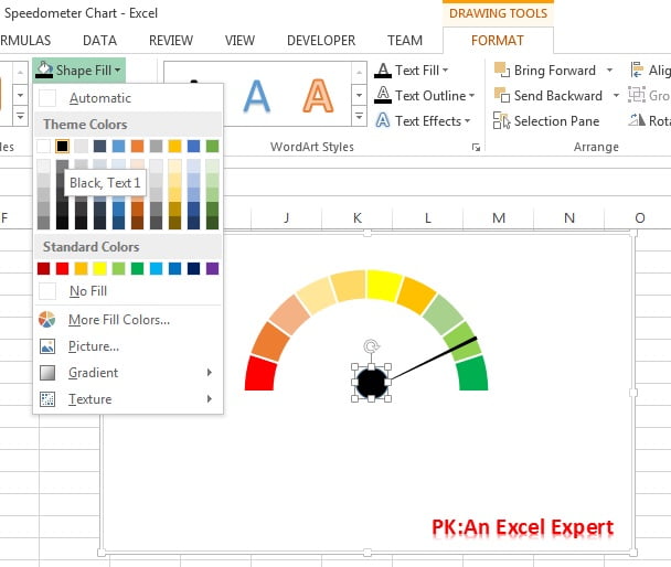
Speedometer Chart - PK: An Excel Expert
How to Create a Pie Chart in Excel | Smartsheet To create a pie chart in Excel 2016, add your data set to a worksheet and highlight it. Then click the Insert tab, and click the dropdown menu next to the image of a pie chart. Select the chart type you want to use and the chosen chart will appear on the worksheet with the data you selected.

How to Make a Pie Chart in Excel (Only Guide You Need) | ExcelDemy
How to Make a PIE Chart in Excel (Easy Step-by-Step Guide) Here are the steps to format the data label from the Design tab: Select the chart. This will make the Design tab available in the ribbon. In the Design tab, click on the Add Chart Element (it's in the Chart Layouts group). Hover the cursor on the Data Labels option. Select any formatting option from the list.
How do I change the order of pie chart slices?
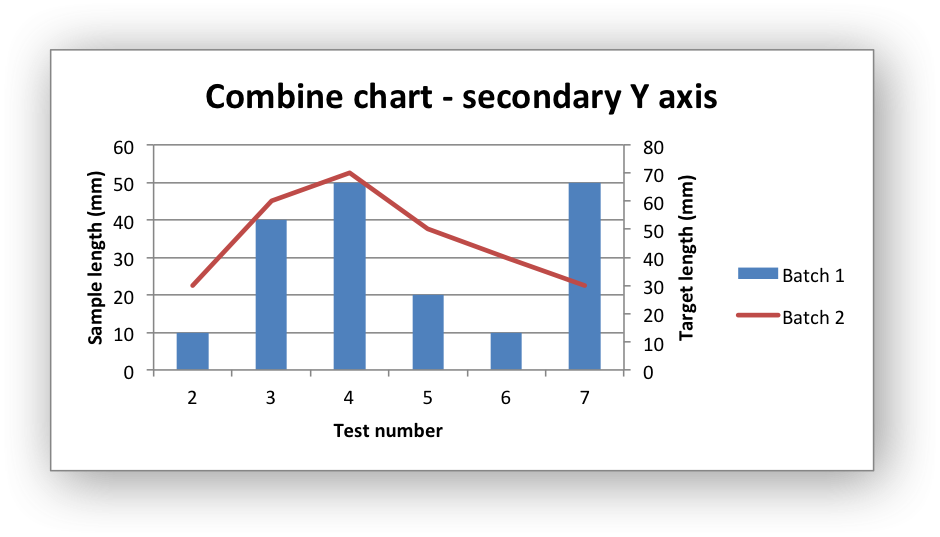
Example: Combined Chart — XlsxWriter Documentation
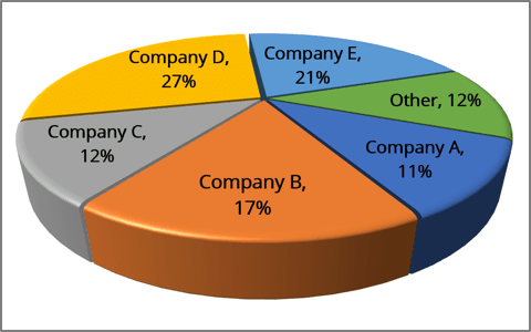
Excel 3-D Pie charts - Microsoft Excel undefined

37 Label Pie Chart Excel - Labels 2021

How to Label a Pie Chart in Excel | It Still Works
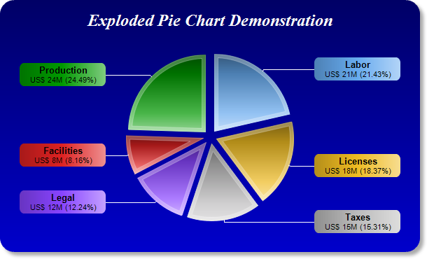
Exploded Pie Chart

Create a Pie Chart in Excel - Easy Excel Tutorial
How to Make a Pie Chart in Excel & Add Rich Data Labels to The Chart!
How to Create a Pie Chart in Excel | Smartsheet

Creating Pie Chart and Adding/Formatting Data Labels (Excel) - YouTube

Microsoft Excel Tutorials: Add Data Labels to a Pie Chart

How to Make a Pie Chart in Excel & Add Rich Data Labels to The Chart!
Automatically Group Smaller Slices in Pie Charts to one big Slice | Chandoo.org - Learn ...
Post a Comment for "43 pie chart excel labels"