42 add labels to bar chart excel
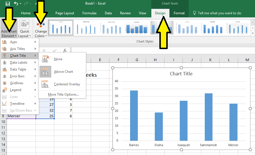
How to Add a Line to a Chart in Excel - Excelchat In order to add a horizontal line in an Excel chart, we follow these steps: Right-click anywhere on the existing chart and click Select Data. Figure 3. Clicking the Select Data option. The Select Data Source dialog box will pop-up. Click Add under Legend Entries. Figure 4. Excel charts: add title, customize chart axis, legend and data labels Click anywhere within your Excel chart, then click the Chart Elements button and check the Axis Titles box. If you want to display the title only for one axis, either horizontal or vertical, click the arrow next to Axis Titles and clear one of the boxes: Click the axis title box on the chart, and type the text.
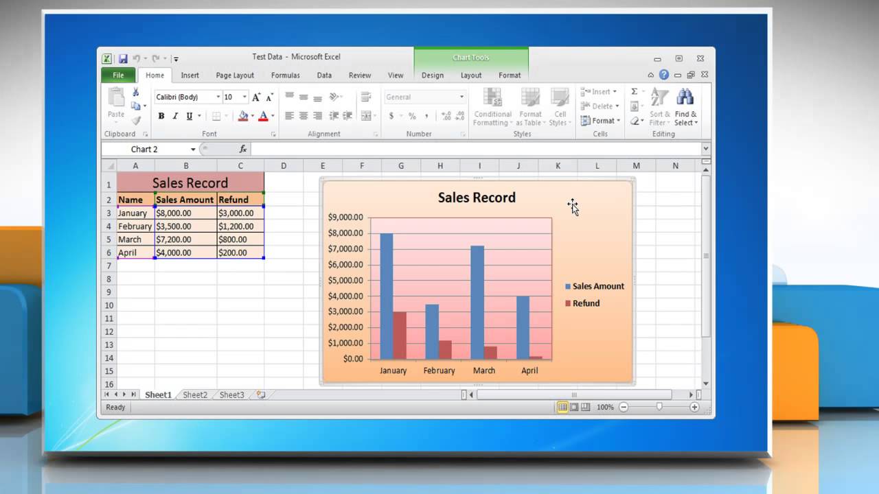
How to Add Data Labels to an Excel 2010 Chart - dummies Use the following steps to add data labels to series in a chart: Click anywhere on the chart that you want to modify. On the Chart Tools Layout tab, click the Data Labels button in the Labels group. A menu of data label placement options appears: None: The default choice; it means you don't want to display data labels.

Add labels to bar chart excel
How to Add Axis Labels in Excel Charts - Step-by-Step (2022) - Spreadsheeto Left-click the Excel chart. 2. Click the plus button in the upper right corner of the chart. 3. Click Axis Titles to put a checkmark in the axis title checkbox. This will display axis titles. 4. Click the added axis title text box to write your axis label. Or you can go to the 'Chart Design' tab, and click the 'Add Chart Element' button ... How to Insert Axis Labels In An Excel Chart | Excelchat We will again click on the chart to turn on the Chart Design tab We will go to Chart Design and select Add Chart Element Figure 6 - Insert axis labels in Excel In the drop-down menu, we will click on Axis Titles, and subsequently, select Primary vertical Figure 7 - Edit vertical axis labels in Excel Edit titles or data labels in a chart - Microsoft Support On a chart, click the label that you want to link to a corresponding worksheet cell. On the worksheet, click in the formula bar, and then type an equal sign (=). Select the worksheet cell that contains the data or text that you want to display in your chart. You can also type the reference to the worksheet cell in the formula bar.
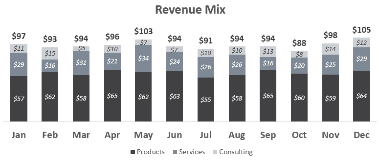
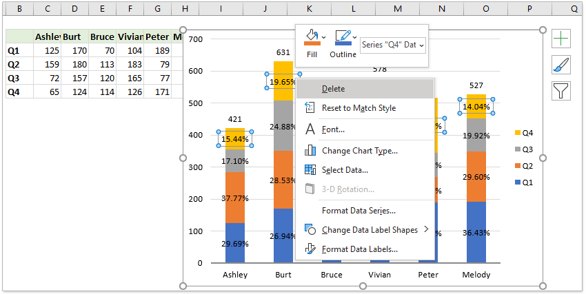
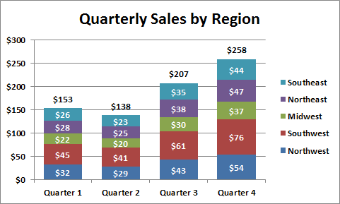
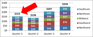
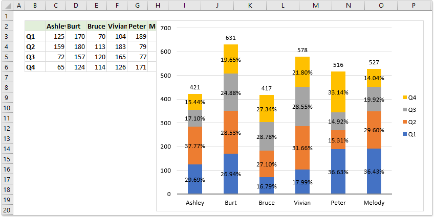
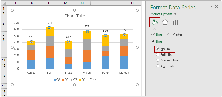
Add labels to bar chart excel. How to Add Total Values to Stacked Bar Chart in Excel In the new window that appears, click Combo and then choose Stacked Column for each of the products and choose Line for the Total, then click OK: The following chart will be created: Step 4: Add Total Values Next, right click on the yellow line and click Add Data Labels. The following labels will appear: Next, double click on any of the labels. How to Show Percentage in Bar Chart in Excel (3 Handy Methods) - ExcelDemy 📌 Step 02: Insert Stacked Column Chart and Add Labels Secondly, select the dataset and navigate to Insert > Insert Column or Bar Chart > Stacked Column Chart. Similar to the previous method, switch the rows and columns and choose the Years as the x-axis labels. Next, go to Chart Element > Data Labels. How to place labels underneath bar chart - Microsoft Community The names are appearing below the chart axis, that is on value 0.0%. They are on the correct place. If you want them to appear at the bottom of your chart, just select the axis and on the "Format axis" dialog box, on the "Axis options" tab, on the "Axis labels:" option, select "Low". jpgpinto jpgpinto Bar Chart in Excel (Examples) | How to Create Bar Chart in Excel? - EDUCBA Right, click on the first bar > go to Fill > Gradient Fill and apply the below format. Step 8: To give the Chart Heading, go to layout>Chart Title > Select Above chart. Chart Heading will be displayed as here it is Sales by Region. Step 9: To add Labels to the bar Right click on bar > Add Data Labels; click on it. Data Label is added to each bar.
How to add or move data labels in Excel chart? - ExtendOffice To add or move data labels in a chart, you can do as below steps: In Excel 2013 or 2016 1. Click the chart to show the Chart Elements button . 2. Then click the Chart Elements, and check Data Labels, then you can click the arrow to choose an option about the data labels in the sub menu. See screenshot: In Excel 2010 or 2007 Excel Waterfall Chart Template - Corporate Finance Institute Change Chart Title to "Free Cash Flow." Remove gridlines and chart borders to clean up the waterfall chart. Step 3 - Add Data Labels to the Bars and Columns. Recall that we created a column called Data label position; this column will be used to define the position of the labels. Right-click on the waterfall chart and go to Select Data. Text Labels on a Horizontal Bar Chart in Excel - Peltier Tech Excel 2007 has no Ratings labels or secondary horizontal axis, so we have to add the axis by hand. On the Excel 2007 Chart Tools > Layout tab, click Axes, then Secondary Horizontal Axis, then Show Left to Right Axis. Now the chart has four axes. We want the Rating labels at the bottom of the chart, and we'll place the numerical axis at the ... Multiple Data Labels on bar chart? - Excel Help Forum Select A1:D4 and insert a bar chart. Select 2 series and delete it. Select 2 series, % diff base line, and move to secondary axis. Adjust series 2 data references, Value from B2:D2. Category labels from B4:D4. Apply data labels to series 2 outside end. select outside end data labels and change from Values to Category Name.
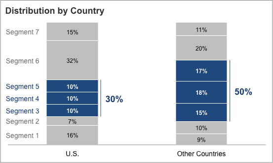
How to Make a Bar Chart in Microsoft Excel - How-To Geek To add axis labels to your bar chart, select your chart and click the green "Chart Elements" icon (the "+" icon). From the "Chart Elements" menu, enable the "Axis Titles" checkbox. Axis labels should appear for both the x axis (at the bottom) and the y axis (on the left). These will appear as text boxes. How to Add Percentages to Excel Bar Chart We will select range A1:C8 and go to Insert >> Charts >> 2-D Column >> Stacked Column: Once we do this we will click on our created Chart, then go to Chart Design >> Add Chart Element >> Data Labels >> Inside Base: Our chart will look like this: Add or remove data labels in a chart - Microsoft Support In the upper right corner, next to the chart, click Add Chart Element > Data Labels. To change the location, click the arrow, and choose an option. If you want to show your data label inside a text bubble shape, click Data Callout. To make data labels easier to read, you can move them inside the data points or even outside of the chart. Stacked bar charts showing percentages (excel) - Microsoft Community What you have to do is - select the data range of your raw data and plot the stacked Column Chart and then. add data labels. When you add data labels, Excel will add the numbers as data labels. You then have to manually change each label and set a link to the respective % cell in the percentage data range.
data visualization - How do you put values over a simple bar ...
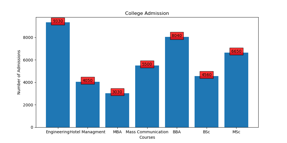
HOW TO CREATE A BAR CHART WITH LABELS INSIDE BARS IN EXCEL - simplexCT 1. Highlight the range A5:B16 and then, on the Insert tab, in the Charts group, click Insert Column or Bar Chart > Clustered Bar. The chart should look like this: 2. Next, lets do some cleaning. Delete the vertical gridlines, the horizontal value axis and the vertical category axis. 3.
Add Total Value Labels to Stacked Bar Chart in Excel (Easy)
How to Make a Bar Graph in Excel: 9 Steps (with Pictures) - wikiHow To do so, click the A1 cell, hold down ⇧ Shift, and then click the bottom value in the B column. This will select all of your data. If your graph uses different column letters, numbers, and so on, simply remember to click the top-left cell in your data group and then click the bottom-right while holding ⇧ Shift. 2 Click the Insert tab.

Aligning data point labels inside bars | How-To | Data ...
How to add data labels from different column in an Excel chart? Right click the data series in the chart, and select Add Data Labels > Add Data Labels from the context menu to add data labels. 2. Click any data label to select all data labels, and then click the specified data label to select it only in the chart. 3.
Graphing with Excel - BIOLOGY FOR LIFE
How to add data labels to a Column (Vertical Bar) Graph in ... - YouTube Get to know about easy steps to add data labels to a Column (Vertical Bar) Graph in Microsoft® Excel 2010 by watching this video.Content in this video is pro...
Labeling a Stacked Column Chart in Excel - PolicyViz
Add Total Value Labels to Stacked Bar Chart in Excel (Easy) Click the Select Range button and select the cell range that contains the total values for your stacked bar chart. After you have confirmed your selection, you should see the label values change to the total bar values in the Excel chart. Format Changes To Your Stacked Bar Chart Remove The Chart Series Fill Color

How to Add Data Labels to your Excel Chart in Excel 2013
How to Add Two Data Labels in Excel Chart (with Easy Steps) 4 Quick Steps to Add Two Data Labels in Excel Chart Step 1: Create a Chart to Represent Data Step 2: Add 1st Data Label in Excel Chart Step 3: Apply 2nd Data Label in Excel Chart Step 4: Format Data Labels to Show Two Data Labels Things to Remember Conclusion Related Articles Download Practice Workbook

How to Add Two Data Labels in Excel Chart (with Easy Steps ...
Adding rich data labels to charts in Excel 2013 To add a data label in a shape, select the data point of interest, then right-click it to pull up the context menu. Click Add Data Label, then click Add Data Callout . The result is that your data label will appear in a graphical callout. In this case, the category Thr for the particular data label is automatically added to the callout too.

Custom data labels in a chart
Add Totals to Stacked Bar Chart - Peltier Tech In Label Totals on Stacked Column Charts I showed how to add data labels with totals to a stacked vertical column chart. That technique was pretty easy, but using a horizontal bar chart makes it a bit more complicated. In Add Totals to Stacked Column Chart I discussed the problem further, and provided an Excel add-in that will apply totals labels to stacked column, bar, or area charts.

How to Add Two Data Labels in Excel Chart (with Easy Steps ...
How to Add Total Data Labels to the Excel Stacked Bar Chart Step 1: Create a sum of your stacked components and add it as an additional data series (this will distort your graph initially) Step 2: Right click the new data series and select "Change series Chart Type…" Step 3: Choose one of the simple line charts as your new Chart Type Step 4: Right click your new line chart and select "Add Data Labels"
How to add total labels to stacked column chart in Excel?
HOW TO CREATE A BAR CHART WITH LABELS ABOVE BAR IN EXCEL - simplexCT In the chart, right-click the Series "Dummy" Data Labels and then, on the short-cut menu, click Format Data Labels. 15. In the Format Data Labels pane, under Label Options selected, set the Label Position to Inside End. 16. Next, while the labels are still selected, click on Text Options, and then click on the Textbox icon. 17.

Add Total Values for Stacked Column and Stacked Bar Charts in ...
Edit titles or data labels in a chart - Microsoft Support On a chart, click the label that you want to link to a corresponding worksheet cell. On the worksheet, click in the formula bar, and then type an equal sign (=). Select the worksheet cell that contains the data or text that you want to display in your chart. You can also type the reference to the worksheet cell in the formula bar.

How to add total labels to stacked column chart in Excel?
How to Insert Axis Labels In An Excel Chart | Excelchat We will again click on the chart to turn on the Chart Design tab We will go to Chart Design and select Add Chart Element Figure 6 - Insert axis labels in Excel In the drop-down menu, we will click on Axis Titles, and subsequently, select Primary vertical Figure 7 - Edit vertical axis labels in Excel
How to Add Totals to Stacked Charts for Readability - Excel ...
How to Add Axis Labels in Excel Charts - Step-by-Step (2022) - Spreadsheeto Left-click the Excel chart. 2. Click the plus button in the upper right corner of the chart. 3. Click Axis Titles to put a checkmark in the axis title checkbox. This will display axis titles. 4. Click the added axis title text box to write your axis label. Or you can go to the 'Chart Design' tab, and click the 'Add Chart Element' button ...

Add data labels and callouts to charts in Excel 365 ...

How to Add Total Data Labels to the Excel Stacked Bar Chart ...
How to add data labels to a Column (Vertical Bar) Graph in Microsoft® Excel 2010
How to add live total labels to graphs and charts in Excel ...

How to use data labels in a chart

Stagger long axis labels and make one label stand out in an ...

Google Workspace Updates: Get more control over chart data ...
How to Add Totals to Stacked Charts for Readability - Excel ...
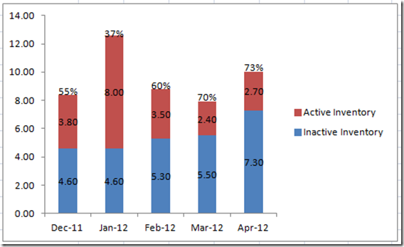
How-to Put Percentage Labels on Top of a Stacked Column Chart ...
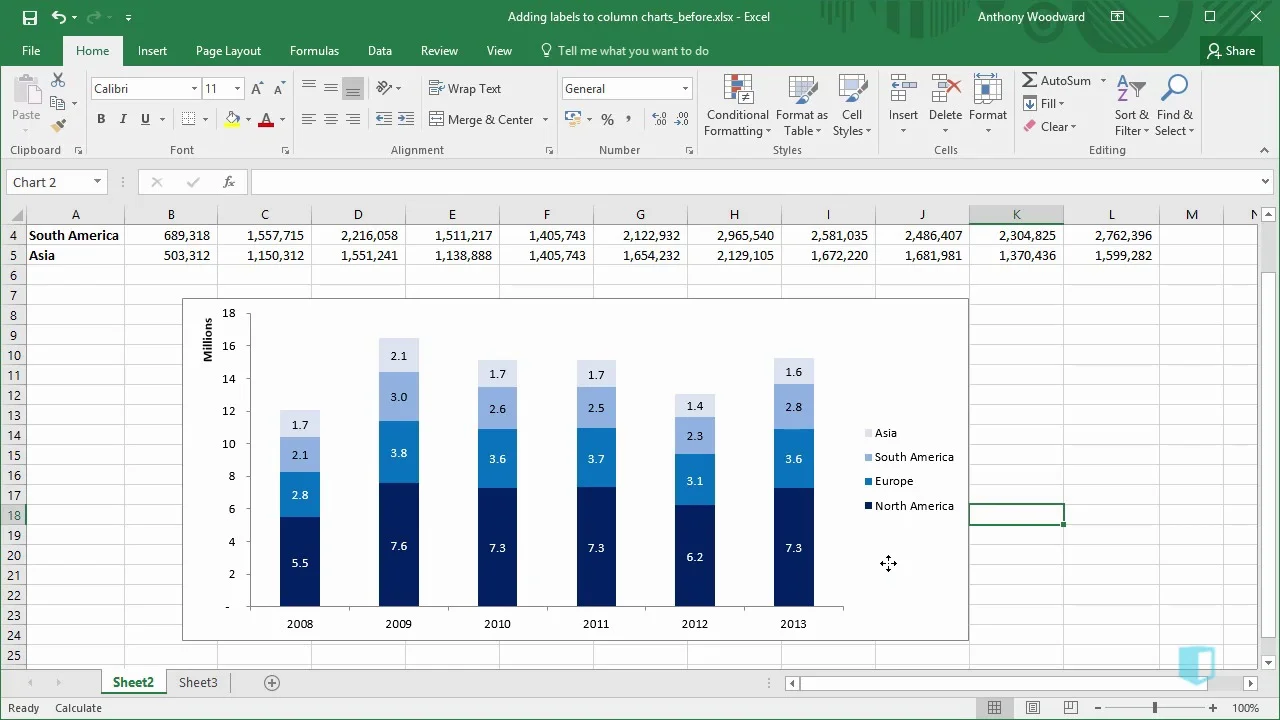
Adding Labels to Column Charts | Online Excel - KPMG Tax - Digital Now Course Training

Adding rich data labels to charts in Excel 2013 | Microsoft ...

How to add data labels from different column in an Excel chart?
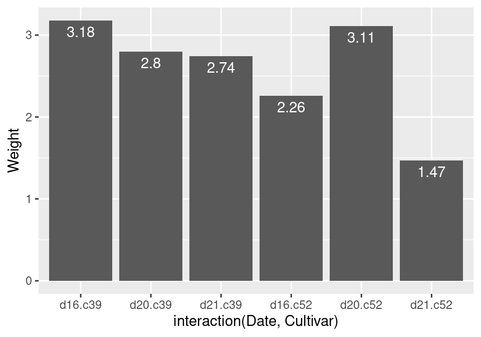
3.9 Adding Labels to a Bar Graph | R Graphics Cookbook, 2nd ...

Stacked column chart in Excel with the label of x-axis ...

Count and Percentage in a Column Chart

Add Labels ON Your Bars
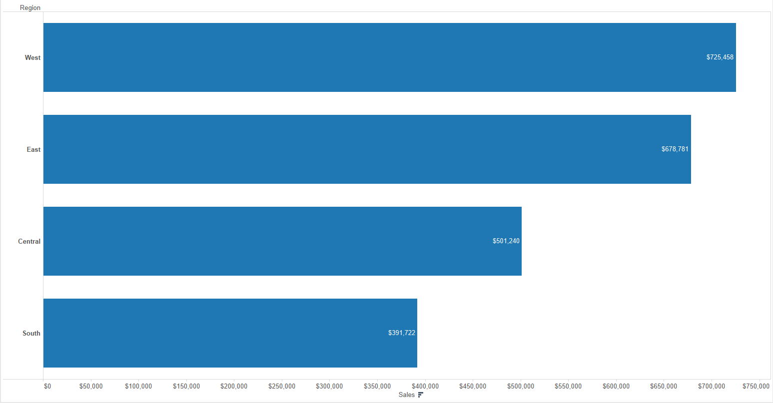
The Data School - Two ways to add labels to the right inside ...
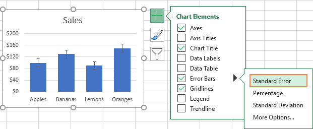
Error bars in Excel: standard and custom
Move and Align Chart Titles, Labels, Legends with the Arrow ...
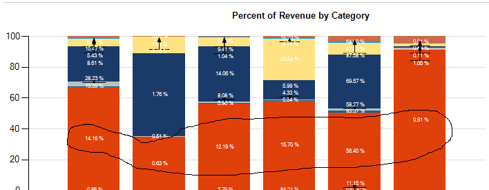
Percentages as Labels for Stacked Bar Charts | SQL Server ...

How to add live total labels to graphs and charts in Excel ...

Add Total Values for Stacked Column and Stacked Bar Charts in ...
Adding value labels on a Matplotlib Bar Chart - GeeksforGeeks

Bar charts with long category labels; Issue #428 November 27 ...
How to add total labels to stacked column chart in Excel?
How to add total labels to stacked column chart in Excel?
/simplexct/images/BlogPic-t005a.png)
How to Create a Bar Chart With Labels Inside Bars in Excel

Adding rich data labels to charts in Excel 2013 | Microsoft ...

Add Data Labels for Total to Stacked Columns in #Excel | wmfexcel
Post a Comment for "42 add labels to bar chart excel"